Flask is a package that can be downloaded onto the Pi along with Flask-Admin. Flask ties in your .py scripts with .html and .css scripts for you to interpret the database generated by Peewee and add it to a web server hosted locally by the Pi. Flask-Admin is an extension of Flask that makes it easier to format and add functionality to your web page using built in functions (that are demonstrated in code below) that will automatically generate blocks of html code for you. It is particularly helpful with databases because it lets you group together all of the usual Create, Read, Update, Delete (CRUD) view logic into a single, self-contained class for each of your models.
Further information on Flask and Flask-Admin can be found by clicking on the respective links.
upv_app.py
from flask import Flask , render_template
from flask_admin import Admin
from flask_admin.contrib.peewee import ModelView

import model

app = Flask(__name__)
admin = Admin(app, name = 'UPV Wind Data',template_mode='bootstrap3',url='/')

app.config['SECRET_KEY'] = 'DIT123' # Have to set secret key or else you won't be able to save things later on.
app.config['MODEL'] = model.SensorAccess()

if __name__ == '__main__':
    app.run(debug=True, host='0.0.0.0')
The code above in ‘upv_app.py’ is the working script that runs your server, it has to be running to access the server. Within the script you can edit the site name and the site template, Bootstrap3 was used as our template style as it has the icest look to it in our opinion. It also points flask in the direction of the SensorAccess object from ‘model.py‘ so that we can include our database on the web page that is generated.
index.html
{% extends 'admin/master.html'%}
{% block body %}
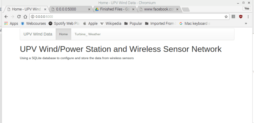
<h1> UPV Wind/Power Station and Wireless Sensor Network</h1>
Using a SQLite database to configure and store the data from wireless sensors
{% endblock %}
<span id="mce_SELREST_start" style="overflow:hidden;line-height:0;"></span>
Above is the ‘index.html‘ script that uses a mixture of jinja(a language that flask-admin uses) and html language to enable a simple way of formatting the web page. Our web page is very simple so there is only a heading 1 and paragraph included.
The output of the ‘upv_app.py‘ and ‘index.html‘ comes out with the basic web page below;
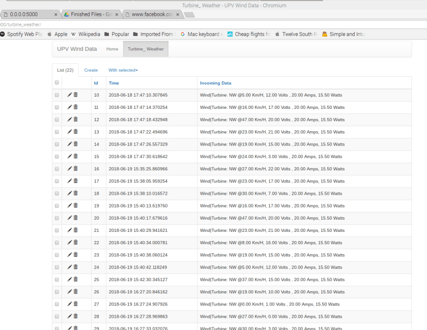
Flask-Admin helped generate interactive tabs such as the Turbine_Weather tab which is a page that displays a table containing our database data as can be seen below;
As Discussed in the post Using an ORM Tool for SQLite , we used the Peewee ORM to act as an intermediate layer between our SQLite database and our Python code.
Model.py
When starting off with SQLite you would create,access and edit your database as shown in the SQLite Database post. With Peewee this process is made a lot easier. A ‘model.py’ file was created. The code from within this file is shown and explained below;
from peewee import * # Imports all the libraries from the Peewee

db = SqliteDatabase('UPVSite.db')# Creates a database(db) called UPVSite.db
''' Standard convention would be to have a Plural as the DB name and singular for the class name(s)'''<span id="mce_SELREST_start" style="overflow:hidden;line-height:0;"></span>

class Turbine_Weather(Model):
      time = DateTimeField()
      incoming_data = TextField()

class Meta:
      database = db
The above code is the start of the ‘model.py‘ script. Apart from what is already commented within the code, it is creating a Model type class named ‘Turbine_Weather‘ that contains the characteristics time and incoming_data, that are declared as a DateTime field and Text field respectively. DateTimeField() and TextField() are two out of a long list of built in field type specifiers within Peewee, a full list can be found at Peewee Field Types . The class named Meta is declaring that the Turbine_Weather Model will have Peewee’s database characteristics which will be important for use with Flask and Flask-Admin later on.
class SensorAccess(object):

# Initialises access to the database
def __init__(self): ''' Self stops confusion between SQLite syntax that is similar to Python syntax '''
    db.connect() # Connects to database
    db.create_tables([Turbine_Weather], safe=True) # Checks if table is made

# Function to add data readings to db table
def add_reading(self,time, incoming_data):
    Turbine_Weather.create(time = time, incoming_data = incoming_data )

# Function to return data correlating to a specific time passed to in
def get_(self, time ):
    data_at_time = Turbine_Weather.get(Turbine_Weather.time == time)
    return data_at_time

# This is a function to return all rows of data
def get_readings(self):
    return Turbine_Weather.select()

# Function to return the latest data readings up to a certain limit in
# descending order
def get_recent_readings (self , limit = 30):
    return Turbine_Weather.select() \
                      .order_by(Turbine_Weather.time.desc()) \
                      .limit(limit)

# Closes the connection to the database
def close(self):
    db.close()
The above code is the final part of the ‘model.py‘ script. Here an Object type class is being made named ‘SensorAccess’. This class contains all functions that will relate to the sensor and related databases, although in this case we only have one db associated with the sensor object. All database query’s are made as functions e.g. get_recent_readings(self, limit = 30).
SerialRead.py
In our case to use Peewee to add the data coming in through the antennas connected to the serial port of the PI a second .py script was needed, we named it as ‘SerialRead.py‘. This script is very similar to the code that was implemented in the Saving Data to a .CSV post. It updates on that by using the functionality within the ‘model.py‘ to add the incoming data sent from the STM32L4 chip to the UPVSite database.
import sqlite3
import time
import datetime
import serial
import string

import model

print ("Starting... ")

ser_in = serial.Serial(port = '/dev/ttyS0', # ttyS0 is for the RPi 3
                    baudrate = 19200,
                    parity = serial.PARITY_NONE,
                    stopbits = serial.STOPBITS_ONE,
                    bytesize = serial.EIGHTBITS,
                    timeout = 100)
print ("Connecting... ")
data = model.SensorAccess()

try:
    while True :

        si = ser_in.readline().strip() # si = Serial in<span id="mce_SELREST_start" style="overflow:hidden;line-height:0;"></span>
        read_time = datetime.datetime.now()#reads in current time into read_time

        print(si)
        data.add_reading(read_time, si)# Adds the current time and incoming data

        time.sleep(300)# Sleeps for 5 minutes before updating its readings
In the code above the data is read in as usual. The major difference is the ‘data.add_reading(read_time, si)’ that uses the ‘add_reading(self, time)’ function within our ‘model.py‘ to add read in data to the database.
We’re using an ORM because it allows the database to be accessed far easier via Python. The Python ORM we’re using is peewee (you read that correctly), it adds a level of abstraction to the process making it far easier to add columns to the database. This is all done by setting up a Python class with the columns being set up just like private variables in a normal class.
General Function of an ORM
To begin using peewee I followed a YouTube tutorial which detailed the general set up of everything: https://www.youtube.com/watch?v=bLO8G21z8bY
When writing the script the classes were initialized in one Python file and the code was implemented in a second.
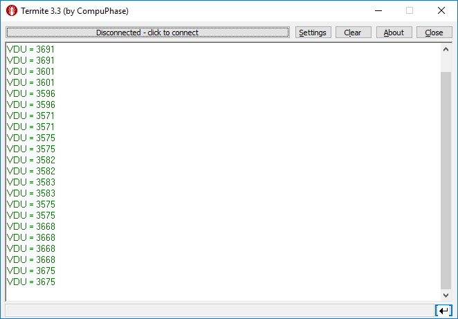
When using the Cortex L4’s ADC, we encountered problems with the consistency of the DU (digital units) being read on Termite (Hyperterminal). In our testing, a steady voltage was sent into the Power Measurement circuit which then dropped our 4 – 24V scale to a 0 – 3.3V, which is a far more suitable range for the MCU. When reading the values from the voltage from the DMM (Digital Multimeter) the values seemed to match those seen in previous tests but when the analogue voltage was converted to DU, the readings were unreliable and had errors up to 350mV.
The power supply seems to be supplying a reliable voltage to the power module, but to make sure we connected an oscilloscope at the two terminals of the supply shown above.
DU Readings at 6VDC
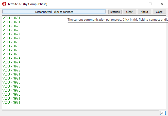
The readings above show the result of sending a constant 6V DC supply into the Power Measurement circuit, the first line is the DU value and the second is DU converted back to voltage to be used to calculate the power. As shown, the DU ranges from 3571 to 3675, a difference of 104.
Assuming a DU range of 0-4095 (12-bit ADC) and a voltage range of 0-24V, these values cause an error of 507mV, an unacceptable error.
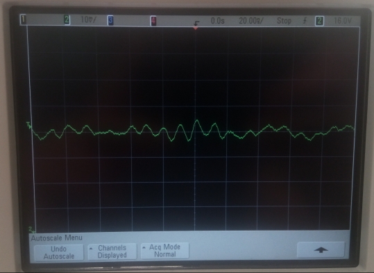
Power Module Ripple
On the top left of the monitor, the voltage scale is shown, each of the verticle lines, in this case, represent 50mV. The oscilloscope shows that the voltage can oscillate between +90mV to -100mV, this explains the large DU jumps when reading from Termite. This wave is also very hard to read due to the large spike only occurring for a very short amount of time.
To ensure the power supply was not at fault we connected the power supply unit to the oscilloscope, spikes either side of the x-axis represent the degree to which the size of the ripple voltage.
Power Supply Ripple
The biggest ripple shown above is less than +/- 5mV, this error is acceptable for our application. This suggests that the power module is at fault and not the power supply.
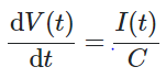
To smooth the output of the power module a capacitor was used, this is often used on rectifiers when converting from AC to DC, a ripple voltage remains and must be smoothed. The differential formula below says that the rate of change of voltage is inversely proportional to the capacitance.
So if the capacitance increases the ripple voltage should be attenuated. To test this an 82nF capacitor was added to the output of the power module (before entering the ADC). When testing with the oscilloscope the waveform below was found.
Power Module Ripple with 82nF
This waveform brings the ripple down to roughly +/- 40mV, 50mV better than without the capacitor. Our aim is to have a voltage accurate to within 100mV of the actual voltage so a smaller ripple was necessary. The next capacitor used was 1µF, the waveform below is what was shown on the oscilloscope.
Power Module Ripple with 1µF
This waveform brings the ripple down to roughly +/- 10mV, 80mV better than without the capacitor. The included capacitor has smoothed the input voltage to the ADC which should, therefore, reduce the spikes in DU read on the Hyperterminal.
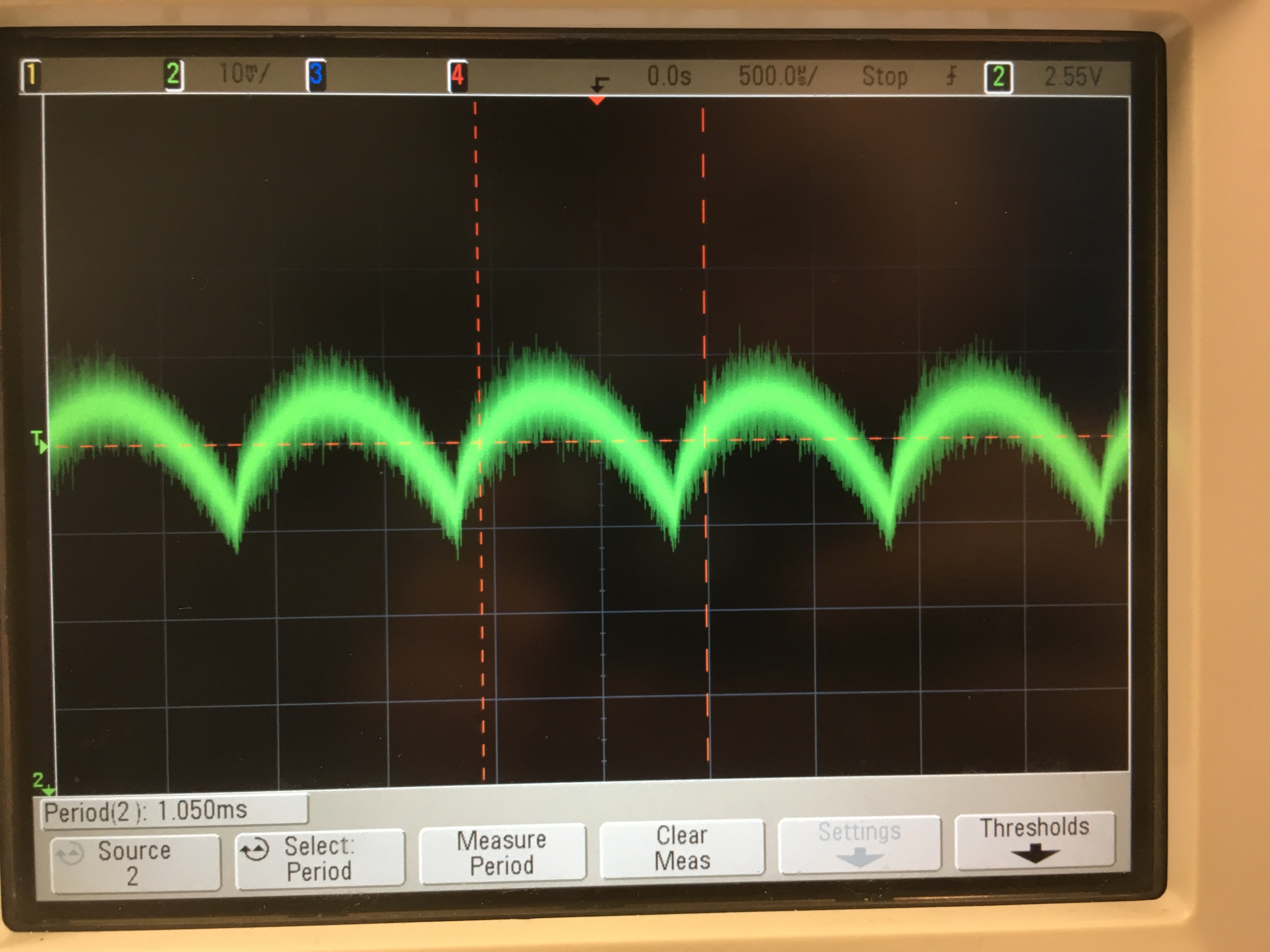
DU Readings with 1µF Capacitor
As shown, the DU ranges from 3661 to 3681, a difference of 20. The values above are an improvement from the non-smoothed output but further work needs to be done to achieve an accurate voltage within 100mV comfortably.
Software Compensation
To further improve the accuracy of the system we can use code to get the average of an array that reads in values from the ADC. First an array of integers must be made to store the DU values. Ideally, an infinite number of elements would be used for accuracy but for low power usage, only 16 elements were used.
int ADC_SamplesV[15], N;
float V_Avg = 0;
for(N = 0; N < 15; N++){
  sConfig.Channel = ADC_CHANNEL_5; // The channel that reads voltage
  HAL_ADC_ConfigChannel(&hadc1, &sConfig);
  ADC_SamplesV [N] = Read_Analog_Value(); // DU is added to the array
  V_Avg += ADC_SamplesV [N]; // the Nth element is added to the variable
  HAL_Delay(1);
}
VDU = V_Avg/N; // finds average of all 16 values
The for loop iterates through the ADC_SamplesV array, where the elements are added to a variable, V_Avg. This is done until it reaches its 15th element where it exits the array and the average is found by dividing the sum of the array, V_Avg, by the length of the array, N.
As seen above, the biggest deviation between the values is 5DU, 15 better than the non-compensated system and almost 100 better than the original.
ADC Reference Voltage
Even with the capacitor on the output and the software compensation, there are still some small, unexplained jumps in DU. One reason for this may be the ADC reference voltage which can have a ripple just like the output of the power module.
In our MCU (Cortex L4), a SAR (Successive Approximation Register) approach is used. For this approach, the input voltage is found by continuously comparing the analogue input to the voltage dictated by the SAR.
SAR Type ADC
If the reference voltage had a ripple of 10mV this would make our reference voltage 3.31V and a given input voltage of 2V would result in an error of approximately 8 digital units. To rectify this problem a capacitor would have to be included just like before, but because these components are within the chip we are unable to solve the problem.
The previous post regarding CSV is useful for local monitoring but in order for it be accessed online the data must be added to an SQLite database. SQL (Structured Query Language) is a programming language which can be understood by a database, it is similar to a CSV in which it stores data in columns and rows but can be accessed more easily by a server. The package sqlite3 must be installed before use.
SQL Basics
The above screen capture is showing basic commands of sqlite3 command line interface. To create a .db file (Database file), the following command is used:
sqlite3 fileName.db
Luckily, SQL is very easy to read and completing tasks that are normally complex in other languages are far easier in SQL due to it being designed with server maintenance in mind, searching the database for a keyword is far faster than say a for loop iterating through the entirety of the data. All commands end with a semicolon, a basic command:
CREATE TABLE – the name of the table follows this command followed by the column details e.g. CREATE TABLE NewTable (Foo REAL, Bar INTEGER);
The data types are also very easy to interpret with int being INTEGER and float being REAL. Contrary to most languages the data type succeeds the variable name which may be confusing.
Although it makes no difference to the function of the code, it is common practice to include the SQL commands/data types (e.g. CREATE, REAL) as upper case, this way when the SQL is included in a Python script it is easily distinguishable. In our server setup, SQL and Python will be used alongside each other as well as the code being shared between two.
import sqlite3
import time
import serial
import string

print ("Starting... ")
serialData = serial.Serial(port = '/dev/ttyS0', # ttyS0 is for the RPi 3
                           baudrate = 19200,
                           parity = serial.PARITY_NONE,
                           stopbits = serial.STOPBITS_ONE,
                           bytesize = serial.EIGHTBITS,
                           timeout = 100)

my_Db = sqlite3.connect('SQL_DB.db')
cursor_Obj = my_Db.cursor()
'''
when selecting stuff in a query, multiple rows are returned so the cursor
remembers where in the query you are
'''

# Storing data from port to database
while True:
  windSpeed, date = t
  reading_time = int(time.time())
  windSpeed = serialData # serial variable read from COM port
  print('Date: {0} windSpeed = {1:0.2f}%'format(date, windSpeed))
  cursor_Obj.execute('INSERT INTO Table1 VALUES (?, ?)',
                    (reading_time, '{0} Wind Speed: ', windSpeed)# finish
  cursor_Obj.commit() # must commit after each
  time.sleep(1) # reads once a second<span
The above code has similar aims to the previous CSV file but with the inclusion of SQL code instead of simply sending the data to a spreadsheet. The use of SQL allows the data to easily managed and transferred. For our project, we are using a particular engine of SQL and that's SQLite, an open source engine which is the most used out of all.
To view the SQLite database in GUI form we used the SQL Studio, available for Windows and Mac for free and is far easier to use than the command line, it also shows the data in a far clearer view.
We added Date along with the two types of information successfully transferred wirelessly from the L4 chip (the MCU we’re using).
A text file is useful for basic data storage and formatting but unfortunately cannot organise the data very well. An alternative to a .txt is CSV file (Comma Separated Values), this allows for the ease of entry of a text file but with the ability to have the data in rows and columns rather than in disarray in normal text.
CSV is similar to a Microsoft Excel file but it can be used in more than just MS Office products making it useful for Linux. A CSV file can be viewed in LibreOffice Calc, a spreadsheet-based program installed by default with Raspbian (Raspberry Pi OS). When data is sent from the Python script it’s commas determine the row and column of where the data is stored.
To store the data with a timestamp the Python datetime module must be used. This allows the Pi to access the current date when storing the data from the serial port. In the code below, a column was made called date and one row was added which contained the current time and date.
import datetime
import csv

time1 = datetime.datetime.now()
time1.strftime("%A %d %b %y %H") # strftime: date formatting

with open('MyCSV.csv', 'w', newline='') as file: # with is a better way to access a file
 write = csv.writer(file)
 write.writerow(['Date'])
 write.writerow([time1])
The screenshot below from LibreOffice shows the result.
Date CSV
The Python script was updated to allow for serial input as well as adding additional columns for future data input such as wind speed and voltage generated by the turbine.
import datetime
import csv
import serial
import string

print ("Starting... ")
serialData = serial.Serial(port = '/dev/ttyS0', # ttyS0 is for the RPi 3
                           baudrate = 19200,
                           parity = serial.PARITY_NONE,
                           stopbits = serial.STOPBITS_ONE,
                           bytesize = serial.EIGHTBITS,
                           timeout = 100)
with open('MyCSV.csv', 'w') as file: # with is a better way to access a file
  write = csv.writer(file)
  write.writerow([' ', 'UPV', 'A. Bailey', 'J. Harding', 'P. Malone'])
  write.writerow([' ']) # adds a blank row
  write.writerow([' ', 'Date', 'Wind Direction', 'Wind Speed', 'Voltage', 'Current', 'Power'])
  write.writerow([' ']) # adds a blank row

while True:
  data = serialData.readline().strip() # Storing incoming data from serial channel to variable "data" and stripping string
  print(data) # displays in the terminal of Pi
  time1 = datetime.datetime.now()
  time1.strftime("%A %d %b %y %H") # strftime: date formatting
  write.writerow([' ', time1, data]) # leaves blank a column
The screen capture below shows all data required to be stored by the turbine in its appropriate columns.
Serial communication has been established between the L4 and the Pi, next is to store the sent data. To do this a knowledge of basic file input/output is needed in addition to the previous PySerial script in the earlier post. The built-in Python function, open(), is used to do this.
import datetime
import serial
import string

print ("Starting... ")
## Serial setup
ser = serial.Serial(port = '/dev/ttyS0',
 baudrate = 19200,
 parity = serial.PARITY_NONE,
 stopbits = serial.STOPBITS_ONE,
 bytesize = serial.EIGHTBITS,
 timeout = 100)

print ("Connected")
x = open("/home/pi/New.txt", "a") # gives directory, "a" is for appending

while True:
 readData = ser.readline().strip() # Storing incoming data in "readData" and stripping string
 x.write(readData) # writes data to variable x, to file New.txt
 x.close()
In the previous post, there were problems with viewing the strings as whole words, the wind direction was being printed as long column of characters which wasn’t very legible so a new function had to be used in PySerial. when reading in the serial data read() was originally used but readline() is a better alternative as it prints the entire transmission.
In the serial set up, a parameter was added called timeout. Timeout determines how long the port reads data, to make it easy the timeout was made to be 100s seconds.
Unfortunately, the other Telit transmitter was being used for other parts of the project so a direct serial connection was made between a laptop via USB. To use a Windows machine to connect, serial connection software must be installed. We used Termite as it’s easy to install and use.
For the next part of this project, we will now focus on the wind turbine. We are required to determine the voltage, current and the power being outputted by the wind turbine. To do this another micro-controller was connected to the power measurement PCB with the necessary components will be used.
The wind turbine generates a voltage between 0 and 24V, to simulate this in the lab a power supply with a 10-ohm load was used. The power measurement PCB has been designed so that it can determine the voltage being generated using an Optocoupler and it can also determine the current by using the ACS758 current sensor. The outputs of the voltage and current are then connected into two separate ADC pins in the chip. From here the power can then be found by calculating the product of the two.
Voltage Measurement
Optocoupler
Firstly, we focused on the voltage component and the SFH6156 Optocoupler. The chip being used can only take a maximum input voltage of 3.3V into the ADC, therefore, something like a voltage divider or a Wheatstone bridge would need to be used in order to obtain a proportional voltage in 0 – 3.3V range. However, since this circuit is required to provide electrical insulation an Optocoupler was used instead.
An Optocoupler is an electronic component that interconnects two separate electrical circuits by means of a light-sensitive optical interface.
The Optocoupler allows you to transmit an electrical signal between two isolated circuits. It has two parts inside the black box, an LED that emits an infrared light and a photosensitive device which detects the light from the LED. When a current is applied to the input the infrared LED begins to emit a light which is proportional to the current. The receiving photosensitive device then switches on and conducts a current the same as an ordinary transistor might.
Enter a caption
For our Optocoupler the input range is 0 – 24V and the output range is 0 – 3.3V however, the relationship between input and output is inversely proportional for our circuit.
Testing
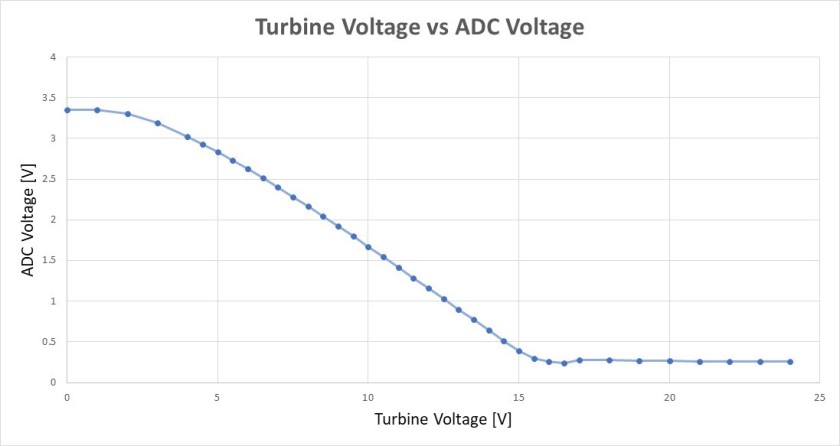
We began testing this component by stepping up the voltage in steps of 1V from the power supply from 0-24V and using the multimeter, we recorded the output of this in a table in excel. We then graphed the relationship of the input of the power source (Turbine) vs the output which would be the input to the ADC as can be seen below.
Turbine Voltage vs ADC Voltage (0-24V)
From this graph, it can be seen that the graph is flat at the beginning but then it starts to transition into a steady slope until it reaches about 16V where it then flattens out and the change in the ADC voltage is minuscule from 16-24V.
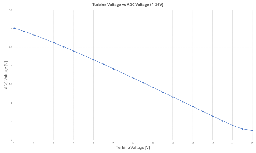
Since we did not design the circuit ourselves as it was designed and built by a previous student, we decided we could only use this module to measure values between 4-16V accurately. This was not a problem for the lower ranges as the minimum voltage the wind turbine would usually produce was roughly 5V so ignoring the inaccuracy of the lower voltages was acceptable. As can be seen in the graph obtained below when the range is reduced, the relationship is much more linear than before however, it is still not perfect.
Turbine Voltage vs ADC Voltage (4-16V)
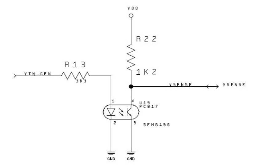
We discussed the results and the limitations of the power module with our project supervisor and during this discussion it was decided that if a larger resistor was used at the input to the optocoupler then this would allow for a wider range of values at the output. This is due to the fact that there would be less voltage and less current going into the input of the opto-coupler when a larger resistor is added. The circuit diagram for the opto-coupler we used can be seen below and we changed the value of R13 from a 3.3KΩ to a 5.6KΩ resistor.
Optocoupler Circuit Diagram
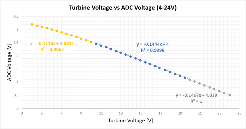
Previously, the change in output voltage of the opto-coupler was miniscule from 16-24V as the opto-coupler had reached a point where the difference in input current made almost no difference to the output current. Therefore, by changing the resistor to a larger value the current was then reduced which allowed for more change in the output current of the opto-coupler. This then led to a larger range of output voltage of the opto-coupler when tested as can be seen in the graph below.
Turbine Voltage vs ADC Voltage (4-24V) With New Resistor
The graph we obtained from our results was far superior to our previous results as we could now measure values from 4-24V. The relationship between the input and output was not completely linear, so we decided that using a piecewise method with several different functions for the different ranges would be a good solution to the problem.
Added 5.6k ohm resistor instead of 3.3k ohm
No capacitor = +- 100mV
added one 82nF nano capacitor(attach images) = +-45
then added 1uF (micro Farad) which worked much better = +-10
period for all roughly 1ms (millisecond)
while (1)
{
   Value = HAL_ADC_GetValue(&hadc1);
   sprintf(aTxBuffer, "Digi<span id="mce_SELREST_start" style="overflow:hidden;line-height:0;"></span>tal Value = %ld \n", Value);
   Mensa_debug_Usart1(aTxBuffer);
   sprintf(aTxBuffer, "S = %d \n \n", S);
   Mensa_debug_Usart1(aTxBuffer);
   HAL_Delay (1000);
   /* USER CODE END WHILE */
}
To upload the data received by the Pi, an HTML server must be set up to pass the weather station information.
from flask import Flask # imports the flask library
from flask import render_template # imports the flask render template
app = Flask(__name__) # sets to default name
app.debug = True

@app.route("/")
def hello(): # making a function called hello
 return render_template('hello.html', message="Hello World!") # passes to hello.html

if __name__ == "__main__": # if name is correct
 app.run(host='0.0.0.0', port=8080) # initiates server at 0.0.0.0 on port 8080
This month we began to make real progress with the Pi, Alex and Phil transmitted the wind direction using a Telit RF transmitter connected to the Cortex L4’s Tx (Transmitting) pin. An identical Telit was on the other side of the lab connected to the Pi’s UART Rx (Receiving) pin.
L4 Chip
To connect the Rx on the Pi, UART had to enabled in the Pi configuration due to it being disabled by default. To change this the following commands were used:
$ cd /boot/  # changes directory to boot

$ ls  # this shows the contents of the boot directory

$ sudo nano config.txt # uses nano to edit config.txt (nano is a text editor in Linux)
At the end of the file UART was enabled: UART = 1, the Pi was restarted to apply changes.
UART: Universal Asynchronous Receiver-Transmitter, part of the computer used to handle asynchronous serial communications.
To wire the Pi, the Tx wire from the Telit was connected to the Rx of the Pi and the Tx of the Pi was connected to Rx of the Telit. Ground was also connected as well as the 3.3V to power the Telit from the Pi.
Pi UART Pinout
To display the serial data on the Pi, pyserial needed to be installed. This followed the same procedure as with other programs. To set up the serial port the following code was used in a Python script.
import serial
ser = serial.Serial( # using the serial library
  port =' /dev/ttyS0', # setting the port as com port 0
  baudrate = 9600, # = transfer rate, must match the L4 setting
  parity = serial.PARITY_NONE, # must match the L4 setting
  stopbits = serial.STOPBITS_ONE, # must match the L4
  bytesize = serial.EIGHTBITS, # usually 7/8, match the L4
  timeout = 5) # determines how long the port is open

print("Connected ") # to tell the user that it's connected

try:
  while True: # infinite loop
    if not ser.in_waiting(): # if the serial port is waiting
      data = ser.read() # variable made equal to what is read
      print data # prints out Rx data in single characters

finally:
  ser.close() #cleanup
The transfer was a success, printing the wind direction as the magnet was moved across the array of sensors on the other end of the transmission. Unfortunately, bytes were being transferred meaning only single characters were received.
The next objective is to receive the data as a string which would be easier to work with and could pass the data to a text or HTML file.